A Conservative and Aggressive Mechanism for Anisotropic Synchrony Convention (CMASC) and (AMASC) Utilizing the Superluminal model from String Theory

Curtis L. Hammitt, Independent Research, Corunna, Indiana 46730.

Keywords: six-day creation, six-day creation time light problem, String Theory, 5D Minkowski space, 4D Minkowski space, 𝝠CDM theory, Lorentz invariant theory

 

Abstract

One of the main arguments against the six-day creation theory is the creation horizon problem, or how light from distant stars and galaxies reaches the Earth in only 6,000 years. Starting in 2011 and going until 2024, there were several peer reviewed papers, (Greene et al. 2011), (Dai and Stojkovic 2024), (Greene et al. 2023), (Greene et, al. 2022) that used String Theory to propose a mechanism for the superluminal propagation of light signals. Including the possibility instantaneous propagation of light without light going faster than the speed of light in its own reference frame. These papers have proposed that this mechanism could solve the Horizon problem in (Lambda Cold Dark Matter theory) 𝝠CDM theory. (Dai and Stojkovic, 2024) Since the 𝝠CDM theory’s Horizon problem is at least similar if not identical to the six-day creation horizon problem these models should also be able to solve the creation horizon problem. The following research uses Greene et al. superluminal theory based on string theory to solve the six-day creation horizon problem. This study’s initial assumption is that the CMB is edge of the universe which Greene et al. in his model calls the “braneworld” and that the redshift from the CMB is caused by the “non-inertial braneworld” moving through an inertial higher dimension that Greene calls the “bulk.” The Anisotropic Synchrony Convention title was used because it proposes a difference in the speed of light in one direction as opposed to the opposite direction. This idea correlates well with Greene et al. braneworld research. This research has shown that Greene et al. “braneworld” model explains not only the general observations in cosmology but also the hard to explain or unexplained observations. Like for example the Axis of Evil,  the redshift limit at z = -1, sometimes called the blue wall and dark energy.

Introduction

In superluminal string theories massless signals are proposed to travel superluminally due to the geometry of compacted dimensions at each point in space in our universe, which is called the braneworld in these theories. String Theory proposes that our universe is made up of up to 11 different dimensions. Most of these dimensions are small compacted dimensions whose circumference can be described by 2𝜋R. In which R is the radius of the compacted dimension, which is generally considered to be a few Planck Lengths in size which is 1x10^-35 m. It is possible that compacted dimensions could be larger, however the arrival time of the light cone is affected by the radius of the compacted dimension which will be shown below. String Theory proposes that light goes “into” these compacted dimensions that are located at every point in the 4D Minkowski space that we inhabit. The theory goes on to propose that our 4D Minkowski space, which is referred to as the braneworld, is embedded and moving in a static larger 5D Minkowski space which is called the bulk that can be thought of as containing the compacted dimensions. In this model time is related to both the 4D Minkowski space or the braneworld and the 5D Minkowski space or the bulk.

If the non-inertial braneworld is moving fast enough when a light signal goes into the inertial bulk space it can appear to move from point A to point B instantaneously because the 4D non-inertial Minkowski space shares the same time dimension as the 5D inertial Minkowski space.  This superluminal travel occurs because of the compacted curled up dimensions that are proposed to exist in our universe “hold” the light while the braneworld that we live in or on moves. In this model, the massless signal never moves at a speed greater than the speed of light in its own reference frame (Dai and Stojkovic, 2024). However, it is proposed in these theories that the 4D Minkowski space does move at a velocity very close to the speed of light. It has been suggested in these cited papers that this would also resolve the horizon problem in 𝝠CDM theory. Greene et al. 2011), (Dai and Stojkovic 2024), (Greene et al. 2023), (Greene et, al. 2022)

Dr. Lisle in his Anisotropic Synchrony Convention (ASC) proposes that when we look out into the night sky, we are seeing the stars in real time (Lisle, 2026). Greene’s et al. theory would agree with this conclusion as long as our braneworld was still moving at a velocity very close to the speed of light (Greene, 2011). This would allow light to effectively travel instantaneously from the deepest regions of the universe. Solving the mechanism issue with ASC, the six day creation horizon issue and 𝝠CDM theory’s horizon issue.

Light traveling faster than light

String theory suggests that both matter and fundamental forces are fundamentally made up of one-dimensional entities called strings, which can take the form of either open or closed strings. Closed strings, often called loops, are distinct from open strings, which are inherently tied to the four or more-dimensional structure of spacetime. The particles that are observe are expressions of open strings, linking them to the fabric of spacetime. These open strings are the essential building blocks of the matter and forces that make up the braneworld. In string theory, light is usually depicted as an open string, linking it to the surface of the braneworld. As a result, like human bodies which are formed from matter and remain connected to the braneworld, so do light signals.

As mentioned above there have been numerous papers published demonstrating the mathematical potential for a massless particle, going from a non-inertial brane-world, to an inertial bulk to traverse these curled-up higher dimensions, making the transmission of light appear superluminal to an observer on the braneworld. In other words, a light signal in the string theory model can have an effective velocity much higher than the speed of light without ever going faster than the speed of light (Greene 2011), (Kabat and Nomura 2023), (Greene 2022), (Greene 2023), (Dai and Stojkovic 2024). Therefore, CMASC and AMASC models described below which are based on these papers do not break any of the foundational equations in relativity.

The CMASC and AMASC models produce effective superluminal velocity, by the braneworld moving very close to the speed of light but still following the Lorentz invariant equation below.

β = v/c   β < 1 (equation 1)

v would be the velocity of our braneworld relative to the bulk. β would represent a fraction of the speed of light. The above equation is from the Lorentz invariant which limits the velocity of the braneworld to a value that is less than the speed of light, c.

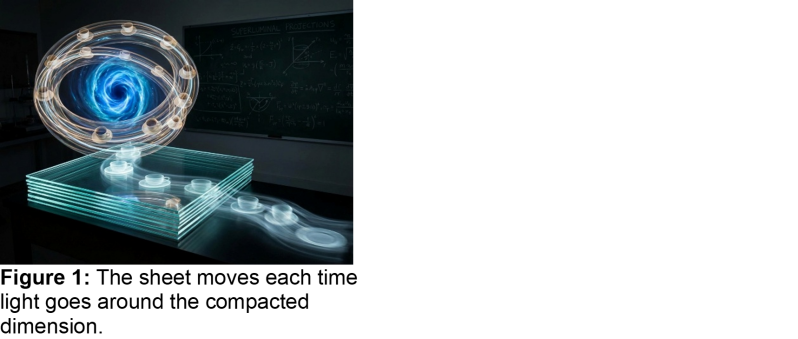
An old trick can be used to describe this superluminal effect. Imagine a table cloth with plates and cups on top of the table cloth. Now imagine a person takes the table cloth and pulls it out from underneath the plates. The plates and cups stay in the same position but the table cloths move underneath the plates and cups. Therefore, the cups and plates can be thought of as effectively coming off of the table cloth and moving into the space above the table cloth. In this example we could describe the table cloth moving relative to the cups and plates. However, there is a critical velocity that must be achieved otherwise the plates and cups remain “attached” to the table cloth because of friction.

This would be similar to how superluminal light is produced except that the cups and plates would revolve around a curled-up dimension. Each time the cup and plate go around the curl up dimension and reach the surface of the sheet it would produce what is called an image on the sheet, which can be interpreted as leaving a picture of the cup and plate on the sheet.  If light that reflected off of a cup at point A and went into the curled-up dimension and the sheet was pulled very quickly then the reflected light ray would reemerge at point B. However, it would appear to an observer on the sheet at B that the image of the cup moved instantaneously from A to B.

Figure 1

Green et al. propose that there is a critical velocity below which light will travel on the surface of the braneworld not leaving the surface. This would be similar to the cups and the plates moving with the table cloth when pulled slowly. However, once the braneworld reaches a certain critical velocity then massless particles can travel in the curled up extra dimensions and take a “shorter” path to the same point (Greene et al. 2023).

Greene et. al. proposes that if a braneworld is not moving with respect to the bulk then the braneworld and the bulk would have Lorentz symmetry. Lorentz symmetry is a fundamental principle of physics stating that the laws of physics remain identical for all observers in inertial frames or frames that are not moving. However, when the braneworld moves at a critical velocity with respect to the bulk then the Lorentz symmetry between the bulk and the braneworld is broken. It is this broken symmetry that allows for the superluminal signal propagation on the brane in a preferred direction. There is a preferred direction because the brane world is moving in one direction and light from the source would expand in all directions. How this preferred direction is related to the “Axis of Evil” is described below. This would cause light to have different effective velocities in different directions This superluminal signal propagation is caused by the speed of the braneworld (β) relative to the bulk. Greene et. al. also showed that effective speed of the signal propagation (c_eff) is described by the Lorentz factor γ. This factor describes how many times faster than the speed of light the braneworld is moving (Greene et al. 2023):

γ = 1/√(1-β²) ≥ 1 (equation 2)

c_eff = γc (equation 3)

Therefore, according to the equations above, superluminal propagation of light can occur by the movement of the braneworld relative to the bulk. If we propose that the universe has a radius of 13.8 billion light years this would indicate for light to take 1 second to reach the Earth from the most distant star 13.8 billion light years away. Light would have to have an effective velocity of 1.296 x 10²⁶ m/s. For light to have an effective speed of 1.290 x 10²⁶ m/s equation 3 shows that γ = 4.33 x 10¹⁷. This would indicate that the velocity of the braneworld would have to be within 4.33 x 10¹⁷ place values of the speed of light. Depending on when God actually introduces the laws of physics into the universe would be an indication of how accurate any theory would be. However, if God accelerated the universe within a tiny fraction of the speed of light superluminal velocity would be possible in this model. If this velocity was maintained, the apparent superluminal propagation would still exist today.

Therefore, a mechanism for superluminal transmission of light at creation could be described in the following manner. God accelerated the universe at Humphrey’s acceleration of 6.67 x 10²⁰ m/s² for a tiny fraction of a second, it would give the universe the background radiation temperature of 2.7 K as shown in Humphrey’s time dilation model (Humphrey 2014). It is estimated that the CMB cools at a rate of 1.87 x 10^-10 kelvins per year. This would indicate that the CMB has cooled 1.12 x 10^-6 K since creation 6000 years ago. The most accurate temperature measurement of the CMB is 2.72548, therefore the CMB has not cooled enough to change the temperature from the original acceleration enough to even measure a change in temperature.  However, the Mechanism for Anisotropic Synchrony Convention (MASC) which is based on the equations of string theory would limit the speed of the braneworld to the speed of light. Therefore, this acceleration could only occur for a maximum of 4.5 x 10^-13 seconds.

The mechanism of superluminal light travel

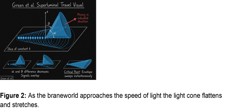
Green et. al. explains superluminal travel of massless particles using the visual representation in the following way and is shown in figure 2. “Blue circles which represent the light cones of images produced by charges on a slice of constant t. The envelope forms a cone with an opening angle ⍺ that moves in the indicated direction, along a line making an angle 𝛳 with respect to the z” axis (Greene et al. 2023).”  Instantaneous travel of light occurs as the difference between angles ⍺ and 𝛳 decrease. As the difference between the two angles decrease the signals begin to overlap and when the geometry reaches a critical point. The envelope becomes so wide and tilted that it sweeps across the braneworld instantaneously.

Figure 2

Imagine the beam of a flashlight as it approaches a wall at an angle < 90֯. As the flashlight approaches the wall the beam spreads out to a point in which the beam stretches all the way across the wall. This would represent when massless particles travel instantaneously. It is because of the potential instantaneous travel of massless particles that many proponents of this theory believe it can solve the horizon problem in the Big Bang theory. However, in relativity, there is no such thing as “the same time” because if an observer has a velocity of any kind or is in a gravitational field of any kind, the observer will have its own characteristic “now" which would be different from every other observer’s now. It is this difference in every observer’s “now” that Dr. Lisle uses in ASC. He defined a different “now” that the speed of light is based on.

The Creation Event

In the theory of Relativity, there is no concept of a "master clock." Relativity indicates that the time experienced by an observer at points A and B, which are far apart, can differ in their perception of what is currently happening. According to Relativity, what an observer considers to be "now" is influenced by their motion and the path that light takes from point A to point B. However, when God created the universe 6000 years ago, there was a unique moment when the entire universe shared the exact same "now." There was no time before t = 0, so the idea of t < 0 did not exist at creation.

The CMACS and the AMACS theories have different creation scenarios because the CMACS model proposes that the effective velocity of light is no longer superluminal. Whereas the AMACS model proposes that the effective velocity of light continues to be superluminal because the braneworld is still moving with respect to the bulk.  Both models would propose that God accelerated the braneworld at Humphrey’s acceleration 6.67 x 10²⁰ m/s² to give the CMB the 2.7255 K temperature. However, the CMACS model has the universe decelerating at -6.67 x 10²⁰ m/s² at the end of day 4 because the braneworld no longer has a velocity with respect to the bulk.

CMACS Model of creation event

In the CMACS model on day 1 of creation God created the bulk and the braneworld and they are static relative to each other. On day 4 God accelerates the braneworld at Humphrey’s acceleration to a point in which γ = 4.33 x 10¹⁷. In other words, the braneworld would be traveling at 4.33 x 10¹⁷ times the speed of light. God creates all of the matter in the universe in a manner similar to Dr. Faulkner's “Dasha” solution (Faulkner 2026). Then at the end of day 4 God decelerated the braneworld so that it now follows the Lambda Cold Dark Matter theory or 𝝠CDM theory. In this model light from the most distant objects reached the Earth in one second and then after the deceleration the light moved according to the equations of 𝝠CDM theory. 

AMACS Model of creation event

On day one of the creation event God created the universe with 4D Minkowski space and the 5D Minkowski space.  The Earth in the 4D Minkowski space. God accelerated the 4D Minkowski space at Humphrey’s blackbody acceleration of 6.67 x 10²⁰ m/s² for less than 4.5 x 10^-13 seconds or until the braneworld reached 99.9998319% the speed of light. This means β would equal 0.999998319. This β value was derived from equation 13 below using the z value of 1089.92 which is the z value of the CMB. Putting this β value into equation 2 means that 𝛾 = 545.46 or that light will have an effective velocity of 545.46 times the speed of light from equation 3. In this model God accelerated the braneworld to 99.9998319% the speed of light and it still has that velocity. Therefore, light can still have the potential to travel instantaneously today.  

For the light to actually arrive on day 4 light would have to have an effective speed much higher than 545.46 times the speed of light. Even at this speed light would still take 24 million years to reach the Earth from the edge of the universe. Therefore, the effective speed of light has to be greater than 545.46 times the speed of light. Green et al. developed this model as a proposal of how communication signals could travel faster than the speed of light in a spaceship that was traveling at a significant percentage of the speed of light.

The motion Greene et al.’s spaceship was described as B which is also a fraction of the speed of light that the spaceship is traveling. The effective speed of a light signal which includes the motion of a moving observer is given by equation 6 below. In order for light the reach the earth the Earth would also have to be moving at a rate of 548 km/s. Earth’s velocity relative to the CMB is estimated at 600 km/s. Therefore 548 km/s is very plausible. If the Earth was moving at 548 km/s then light from a star created on day 4 at the “edge” of the universe reaches the Earth in negligible time on our clocks, because light could have an effective speed over 3.5 million times the speed of light.

The Mechanism CMACS and AMACS

In the CMACS model most of the effective speed of light comes from the velocity of the braneworld in the bulk. When the observer remains stationary all of the effective velocity comes from the non-inertial braneworld moving with respect to the inertial bulk. However, when the observer is moving this movement changes the effective velocity. 

The CMASC theory would have a 𝛾 = 4.33 x 10¹⁷ the corresponding redshift associated with this high 𝛾 would be z = 8.66 x 10¹⁷. This is far outside any possible observed redshift because the highest electromagnetic redshift is 1100. However, this is not outside of theoretically proposed redshifts. Redshift at the proposed end of cosmic inflation was believed to have a redshift of > 10²⁶. A problem with this high redshift is that B_critical=0, which means that any movement on the braneworld would cause the light to go backward in time. 

There are two motions that affect the arrival time of the light from distant stars. The velocity of the braneworld in the bulk and the particular motion of the objects on the braneworld. Equation 4 expresses the velocity in relation to the angles shown in Figure 2.

 v_eff = tan(Θ ± α) / Γβ   (equation 4)

In equation 4, v_eff represents the effective speed of the massless signal moving from point A to point B. Θ indicates the additional tilt angle caused by a moving observer within the braneworld framework. α denotes the opening half-angle of the light cone, mainly influenced by the velocity of the braneworld, and approaches 90° as β approaches 1, or as the braneworld nears the speed of light. In this model, α approaches the speed of light, spreading across the surface of the braneworld. Θ describes the observer's motion and is referred to as the boost, as it adjusts the effective velocity to produce an instantaneous effective velocity. Therefore, Θ ± α reflects the combined effects of both the velocity of the braneworld and that of the observer.

                    (Equation 5) (Greene et. al., 2023)

Equation 5 represents the relationship between the velocity of the observer B and the velocity of the braneworld 𝛽.  B denotes the relative velocity of an observer situated on the braneworld, described as B = v_ob/c. β represents the relative velocity of the braneworld relative to the bulk, defined by β = v_brane/c. As the observer's velocity approaches zero, Tan Θ converges to β, reflecting the relative velocity of the braneworld. We characterize α through the equation sin α = β, yielding α = arcsine β. This angle α is pivotal for comprehending the augmented effective speed of light. As α nears 90 degrees or π/2, the cone expands and flattens. As 𝛾 approaches 4.33 x 10¹⁷, 𝛽 approaches 1 and the arcsine 1 is 90 degrees. This expansion of the cone results in the effective velocity approaching infinity.

At θ = 0, when the observer remains at rest, the angles of the leading and trailing edges of the wavefront are described by the following equation:

Upper envelope or leading-edge blue shifted: θ + α = 0° + α = α

Lower envelope trailing edge redshift: θ – α = 0° – α = –α

The effective velocity when B = 0 is described by equation 6 below and then can be simplified to v_eff = (γ)(1) = (γ)(c) as B goes to 0.

v_eff = γ [(1 + Γ²B²β²) / (1 - Γ²Bγβ²)] (equation 6) 

Γ = 1/√1- B² (equation 7)

            B = v_ob/c (equation 8)

Equation 6 simplifies Equation 4 by capturing the effective velocity of the upper envelope of the light cone. When the denominator of Equation 6 (1 - Γ²Bγβ²) nears zero, the effective velocity approaches infinity. Therefore, the parameters B and β determine the conditions that lead to an infinite effective velocity, indicating that for any specific β, there is a critical value of B that will trigger this infinite effective velocity. This critical B will be explained in the following sections. If the denominator in equation six is set to zero equation 9 is produced and solving the equation for B yields B_critical.

 Γ² B = 1/(γꞵ²) (equation 9) substituting equation 7 into equation 9 gives equation 10. 

            (1/√(1-B²))²(B) = 1/(γꞵ²) (equation 10) solving for B gives

            B = (-γβ² ± √(γ²𝛽⁴+4)) / 2 (equation 11)

When the equation above is used to calculate B_critical, the value is expressed as 0.00183331500017297642. However effective velocity calculations seem to place this value at 0.0018333130017297642. Therefore, the calculated value is 1.09E-4% different than the effective velocity value. The effective velocity value will be used as B_critical.

Since γ is defined as γ = 1/√(1-𝛽²), it follows that for any given 𝛽, the critical B can be determined, and 𝛽 can subsequently be derived from the redshift. Therefore, if the redshift at the CMB is assumed to represent the z value that is produced by the velocity of the braneworld in the bulk the corresponding B value should be able to be determined. The equation for relativistic redshift is presented below.

            1 + z = √((1+𝛽)/(1-𝛽)) (equation 12) Solving equation 12 for 𝛽 gives:

            𝛽 =  (equation 13) Where z is the redshift.

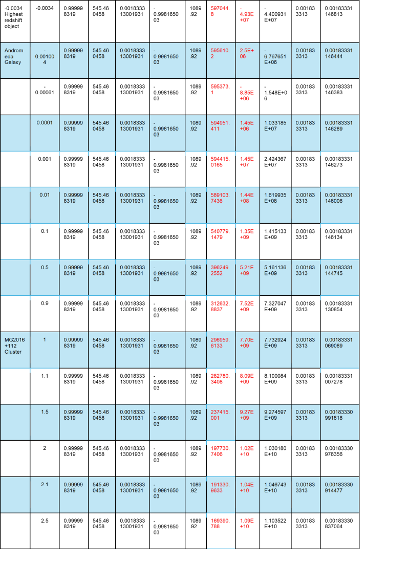
The Cosmic Microwave Background (CMB) has a redshift (z) value of 1089.92. Plugging this z value into equation 13 gives a beta (𝛽) value of 0.9999983194. Using this beta in equation 11 results in a critical B value of 0.0018351317. Applying equation 8 then yields a velocity of 548 km/s. Because the B value is related to the motion of the observer and it is this motion that determines the redshift that we are observing on Earth, all of the B values that are associated with Earth’s particular motion and have B values which are within < 1% of B critical. It would be expected that an observer in the Andromeda Galaxy would calculate a different B value because of the different motion of the Andromeda Galaxy. The estimated velocity of the Earth relative to the CMB is around 370 km/s the galaxy has a velocity of around 552 km/s to 630 km/s. Therefore 548 km/s is a very plausible velocity.

This finding is significant as it is based on braneworld equations developed by Greene et al. Within the braneworld model. In other words, the Earth's velocity is being understood in the context of the braneworld's motion relative to the bulk. In a model where the braneworld moves uniformly, this constant velocity generates the Cosmic Microwave Background (CMB), with redshift serving as a metric for objects in relation to this motion.

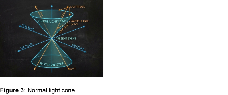
Description of Propagation of light in the Braneworld Model

The braneworld model of the propagation of light still describes a normal light cone. However, it describes how this light cone will change into a light cone that looks like figure 2 as the braneworld or universe approaches the speed of light in a string theory framework. Therefore, the light cone still has a future light cone and a past light cone. However as described above this light cone changes shape as velocity of braneworld changes and as the velocity of the observer changes.

Figure 3

The future and past light cones are referred to as front and trailing envelopes due to their resemblance to an envelope once when they undergo the process of flattening and elongation across the surface of the braneworld as shown in figure 2.  This shape signifies when light possesses an instantaneous effective velocity.

The upper envelope, which contains the initial signals, undergoes a blue shift due to the compression of light rays caused by the velocity of the braneworld. Currently, the majority of stars in the universe exhibit a red shift rather than a blue shift. Nonetheless, both the upper and lower envelopes possess an effective superluminal speed, enabling a potential mixing of blue shifted and redshifted light. This mixing would be influenced by the difference in arrival times between the front envelope and the trailing envelope. Two images are perceived by an observer when the difference in arrival time is long enough. However, if the arrival time difference is sufficiently small, the perception will be of a single image instead of two. Below are the equations that detail the arrival times of the front and trailing envelopes.

t₊ = 2πRw√(1- β)/(1+ β)      Arrival time of blue-shifted light (equation 14)    

t_- = 2πRw√(1+ β)/(1- β)       Arrival time of red-shifted light (equation 15)(Greene et al., 2022)

R = radius of compacted dimension

w = number of time signals go around compacted dimension usually 1

            β = velocity of braneworld relative to the speed of light

Arrival times are determined by the radius of the compacted dimensions. Equation 14 and 15 shows the direct relationship between t and the radius of the compacted dimension. As the velocity of the braneworld relative to the bulk increases, β approaches one, causing the denominator under the radical to approach zero. If the compacted radius is very small, the arrival time will also be very small. When β approaches 1 and w equals 1, it indicates that light has circled the extra dimension once, then equations 14 and 15 simplify to equations 16 and 17.

 t₊ = 2πR(1/2γ) blue shifted (equation 16)

 t_- = 2πRw2γ   redshifted (equation 17)

Therefore, the change in time can be described by equation 18.

            Δt = 2πRw2γ - 2πR(1/2γ) = 4πRwγ (equation 18)

The reason why the equation is equal to 4πRwγ is because when γ is sufficiently large 2πR(1/2γ) can be ignored.

The redshift starts to dominate once the blue shifted image has arrived and begun to fade in its relative impact, allowing enough time for the subsequent redshifted image to become the main source of light that is being received. This happens because the blue shifted flash is compressed in time, while the redshifted light is received over a longer period. According to the CMACS model, when stars and galaxies first formed and their light reached Earth, it was mainly blue-shifted. However, as time went on, the redshifted light became more prevalent. The shift to dominance by redshifted light occurs when its energy level exceeds that of the blue shifted light.

Energy of Red and Blue shifted light

In the AMACS model Δt determines the mixing of the blue shifted light and the redshifted light. Another way to describe the mixing of blue and red shifted light is in equating the energy of each type of light. The type of light that has more energy determines the z value of the light.  The blueshift factor, characterized by a positive winding in the forward direction, is shown in equation 19 which is the Doppler equation

D_b = √(1+𝛽) / (1 - 𝛽) = 2γ (equation 19) for a large 𝛾

            D_b = energy per blue shifted photon

The redshift factor with a negative winding,

            D_r = √(1-𝛽) / (1+ 𝛽) = 1/2γ (equation 20) for large 𝛾

                        D_r = energy for red shifted photons

Equations 19 and 20 are for comparing the energy of the red and blue shifted photons.

Equation 21 is the ratio of energy of blue photons to energy of red photons then would be

            D_b^2: D_r² = 4𝛾² (equation 21)

Equation 21 shows that in this model blue shifted photons have much more energy than red shifted photons and that this energy is dependent on the velocity of the non-inertial reference frame or the braneworld.

In this model the absolute value of the velocity of the trailing envelope does not always equal the velocity of the front envelope. The difference in velocities causes an increasing Δt in the arrival time. The velocity of the front envelope is represented by v_eff and the velocity of the trailing envelope is represented by |ω|. The absolute of ω is used to compare the two velocities because the velocity of the trailing envelope is always in the opposite direction relative to the front envelope.

As shown in equation 18, the temporal delay between the blue shifted and redshifted images is contingent upon the radius of the compactified dimension. This phenomenon arises from the duration required for light to traverse the circumference of the compactified dimension. Consequently, a larger compactified dimension results in an extended Δt. The significance of R in the equation is pronounced, because R is quantified in light-years.

Assume a source emits energy for a brief period, and the observer analyzes the total energy received on the brane. The effective "burst" of blue shifted energy is transmitted within a short duration roughly equal to Δt_b ≈ 2πR/v ≈ 2πR/γ, where γ is quite large. In contrast, the redshifted light reaches the observer more gradually. However, the redshifted images continue to arrive continuously, with successive occurrences happening at intervals of 2πR/ω. In this equation, ω represents the speed of light in the direction opposite to v.

The cumulative energy that is blue shifted shows a quick rise before eventually leveling off at the forward front. However, the cumulative energy that is redshifted keeps rising steadily over time, with more negative-winding modes adding to this buildup. A reasonable equilibrium is attained when the trailing component is given extra time to gather enough energy to balance its lower energy per photon. The crossover time, referred to as t_dominate, can be expressed by the following equation.

(Energy per blue shifted photon) x (effective duration of blue shifted burst) = energy per redshifted photon) x (accumulation time for redshifted)

D_b x (2πR/v) = D_r x t_dominate (equation 22)

Equation 22 is equating the energy of the blue light for a given amount of time to the energy of red light over a given amount of time. Solving the equation for t_dominate gives equation 23 which is the change in arrival time that makes the redshifted light more dominant than the blue shifted light. 

            t_dominante = (D_b/D_r) x 2πR/v (equation 23)

Since (D_b/D_r) = 4𝛾² and v ≈ γ Because R is a distance this the equation in this form is a distance:

 Distance(t_dominante) = 4𝛾² x 2πR/γ = 8πRγ  (equation 24)

This result is assuming that all the blue shifted energy arrives in a very short burst with a duration of 2πR/v, and that the redshifted energy accumulates after this time. In reality, both the forward moving envelope and the trailing envelope are spreading out over time. The trailing component is not waiting completely after the forward burst; the two are overlapping significantly. Estimating the average gives equation 25:

Distance(t_dominante) = 8πRγ/4 = 2πRγ (equation 25) To convert this distance to time, the equation needs to be divided by the speed of light.

t_dominante = 4πRγ/c = 4πRγ/2.99 x 10⁸ m/s (equation 25.5) changes distance to time

            T_dominante = 1.1456 x 10^-40 s When R = 1 x 10^-35 m

The CMB has the highest observed z value which is measured at 1089.92 which is usually estimated to 1100. Equation 13 gives 𝛽 value of 0.99999835 therefore γ = 545.46 that can be calculated from equation 2.

The compacted dimension could be any size but the most commonly cited size in string theory literature is that the compacted dimensions are on the order of plank distances = 1 x 10^-35 m. If this were the case then the Δt would be small enough for only one image to be discernible no matter what type of measuring device is used. 

Redshift without movement of objects in the Universe

In the AMACS model mentioned above, in the absence of any other movement yields a Lorentz factor (γ) of 545.46. Substituting this value into equation 3 results in an effective velocity of 545.46 times the speed of light (c), rather than an instantaneous velocity. Even at this superluminal speed, light from CMB would still require over 24 million years for light to traverse the distance to Earth.

For light to reach Earth without any movement of the planet, γ would need to be the exceedingly high value of 4.33E17, as previously calculated in the CMACS model. This high γ in the CMACS model results in a z value significantly exceeding 1100. This γ would have to be the result of a divine force accelerating the universe to an to a speed that would be with in 4.33E17 place values of the speed of light and then decelerating it back to β = 0.

Because of the ultra-high γ value in the CMACS model the time for T_dominante would increase 17 orders of magnitude over the AMACS model. This would produce a T_dominante = 9.0 s. Therefore, there would have been two different images of the stars and galaxies while God was creating them. If the circumference of the compacted dimensions were larger, Δt would quickly reach a point in which this model would not be tenable in a six-day creation system. 

If the compacted dimensions were a nanometer in size Δt would be 1.4 hours. An observer on the Earth would see a flash of blue light and then everything in the universe would shift towards the red end of the spectrum for 1.4 hours and they would see multiple images of the stars and galaxies that God created. Until God slowed the universe to β = 0. Then redshift would fade away and then the expansion effects of the universe would dictate the redshift of the light. There would be no break in the propagation of light because as β approached zero the light image would move from the compacted higher dimension to our three-dimensional space from the Earth all the way back to the origin of the light.

This type of model could be a mechanism for Dr. Faulkner’s “Dasha” proposal, in which God quickly formed and moved all of the celestial bodies in the universe on day four and then the light from these bodies reached the Earth on day 4. After that the expansion of the universe dictated the z value of light reaching the earth. As God moved the stars and galaxies especially at the high velocities, He would have to move them. The images would have gone backward into time. This does make for an interesting solution to what produced the light before the sun was created. When God started the flow of time light from day four could have produced the light that was produced on day 1.

Redshift with movement of objects in the Universe and the Axis of Evil

In the AMASC model, which is more in line with Dr. Jason Lisle’s ASC proposal, God accelerates the universe at Humphrey’s acceleration. However, He only accelerates the braneworld to an effective velocity of 545.46c which would be 99.9998319% the speed of light. After which the braneworld has maintained the same constant velocity of 99.9998319% the speed of light which persists to this day. In this framework, the CMB redshift results from the constant velocity of the braneworld within the bulk and the motion of objects in the universe. This effective velocity has already been described in equation 6.

v_eff =  γ [(1 + Γ²B²β²) / (1 - Γ²Bγβ²)]

The braneworld’s velocity was determined based on the observed redshift of the CMB, which is z = 1089.92. Using Equation 13, gives a β value of 0.999998319, leading to a 𝛾 value of 545.46 calculated from Equation 2. It was posited that the CMB results from the motion of the braneworld within the bulk. Therefore, The AMACS model proposes that the constant temperature of the CMB stems from the steady velocity of the braneworld traveling through the bulk, as indicated by the redshift of the CMB. The β value derived from the CMB results in a critical B value of 0.001834997, which corresponds to a specific velocity of 548.664 km/s.

In the AMACS model, it is the particular velocity of the Earth and the motion of the braneworld in the bulk that produces the near instantaneous effective velocity of light. B_critical is given by equation 11 above. Any particular velocity that produces a B value that is > B_critical. Produces light signals that go backward into time. Any particular velocity that produces a B value that is equal to B_critical produces an effective speed of light that goes to infinity.

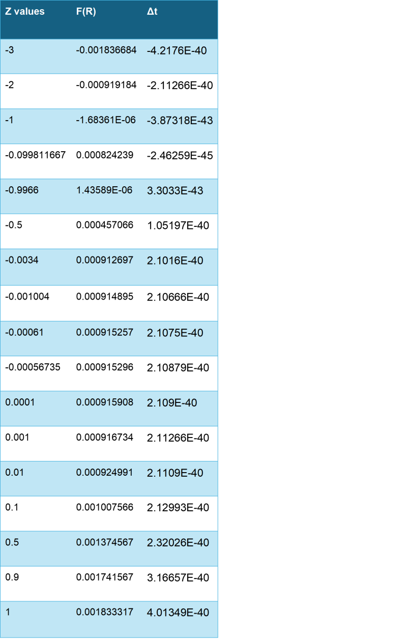
Chart 3

According to AMACS theory, the motion of the Andromeda Galaxy is different from the motion of the Earth. The z values observed in the Andromeda Galaxy would be similar to those seen on Earth because 𝛽 and 𝛾 would be the same. However, the z values would be a little different because the B value would be different because of the different motion of the Andromeda Galaxy.

AMACS would also expect the Andromeda Galaxy to have a different orientation of the Axis of Evil than what is observed on earth. The Axis of Evil would be caused by the difference in arrival times of the front and trailing envelopes which is caused by the velocity of the braneworld 𝛽 and the velocity of a particular observer B.

The "Axis of Evil" is an unexpected, unexplained alignment of large-scale temperature fluctuations in the Cosmic Microwave Background (CMB). It is considered an anomaly because these massive cosmic structures appear to line up with the plane of our Solar System. When the CMB is analyzed and the underlying primordial ripples are examined using mathematical shapes called multipoles. It was discovered that there were two underlying shapes. The Quadrupole, L= 2, that splits the sky into four alternating warm and cool zones, and the Octupole, L=3, splits the sky into eight alternating warm and cool zones.

In 𝝠CDM theory the Axis of Evil is an unexplained anomaly that makes some believe that a new type of physics is needed to explain it. Whereas in AMACS theory the Axis of Evil is a needed observation to confirm AMACS cosmology. In the moving braneworld model, the CMB is not a single uniform surface. Instead, what we observe is a mixture of light from the forward envelope and the trailing envelope, with different properties. The forward envelope is strongly blue shifted and appears hotter or higher temperature. The trailing envelope is strongly redshifted and appears colder or low temperature. Because the two envelopes arrive at different times and with different strengths depending on direction, the sky ends up with temperature variations. This is because the brane is moving which means that the laws of physics on the brane are not the same in all directions. Light does not travel the same way in every direction because of the broken Lorentz invariance. 

A preferred axis is generated because the direction of the brane’s motion plus the Earth’s motion causes the sky to look one way in one direction and in the opposite direction, the sky looks different. This difference creates a global axis across the entire sky. It aligns with the solar system because the Earth has a small velocity component in a particular direction (B). If this direction lines up with the brane’s hidden motion, the preferred axis will appear to point toward the ecliptic plane or our direction of motion which is exactly what is observed in the Axis of Evil.

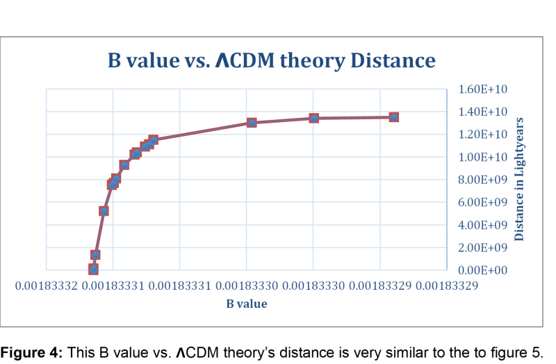
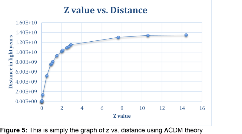
This difference in travel time that causes the axis of evil causes a hyperbola curve, when the redshift is plotted against distance which is shown in figures 4 and 5. It is interesting that the AMACS model gives almost the exact same curve in the opposite direction when B is plotted against distance. B = v_ob/c and B decreases with distance. The boosted speed decreases with distance and this decrease in the observed boosted speed seems to mimic the decrease in redshift per unit of distance.

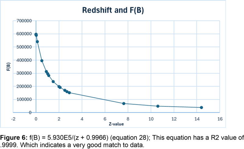
Figure 6 shows the inverse relationship between z_net and the frequency of blue light before mixing with redshifted. This is an inverse relationship because as the blue shifted light decreases as the redshifted light increases. z_net would represent the redshifted light and F(B) would represent the total amount of blue shifted light. So as the redshifted light increases the blue shifted light is going to decrease.

The difference in velocity of the front and trailing envelopes changes the z_net value of the incoming light. Above, it was shown how the top envelope which is blue shifted and the bottom envelope which is redshifted would arrive very close to the same moment when the radius of the compacted dimension was small enough. Especially when the radius was the size of a Planck’s length. Therefore, the red and blue images would be a mixture because of this small difference in arrival time. The difference in arrival time is described in equation 37 below. However, it is shown by chart 1.

Chart 1 

As B approaches B_critical the light is shifted more towards the blue end of the spectrum which is represented by f(B). As shown in chart 2 small changes in B causes large changes in f(B). Because z_net is a mixture of the redshifted and blue shifted light, equation 26 expresses this mixture by weighting the redshifted and blue shifted light differently. The redshift and the blueshift are weighted in a way to indicate the type of arrival of each. The blue shifted light comes in a quick flash and so its weighted to show this time compression (1/𝛾) (f(B). The redshifted light continually arrives after the blue shifted light so the weighted value is 1 to show this sustained delivery. Equation 26 shows the redshift of z_net is controlled by the amount of blue shifted light f(B). Because the redshift is controlled by the amount of blue shifted light. f(B) will be used to convert from z to distance, below.

            z_net = ((w_blue)(z_blue) + (w_red)(z_red))/ (w_blue+w_red) (equation 26)

                        Z_net= the combined or average of blue and red shifted light.

                        𝛾 = 545.46

                        w_blue = (f(B) (1/𝛾)

                        D_blue = 1/𝛾

Z_blue = (D_blue - 1) = -0.998165003

W_red = 1

D_red = 2𝛾

Z_red = (D_red - 1) = 1088.92

Chart 2

This dependence can be seen when the observed redshift is plotted against the full blueshift frequency F(B), it shows an inverse relationship which is described by equation 27.

                        f(B) = 591,714.33/(z +.994)  (equation 27)

Equation 27 was derived by of all of the points in chart 2 except for the CMB. However, the CMB is described by equation 27. In the AMACS model the redshift and blueshift combine to form a whole, as one increases the other decreases. The amount of blue shifted light changes because the velocity of the front and trailing envelope changes. 

The long “tail” that is in figure 8 and not in figure 7 is caused by the high redshift value of the CMB. In the Lambda-CDM model or 𝝠CDM theory, the tail is described as a product of cosmic inflation. This would describe the time when the universe was over a thousand times smaller than it is today and then underwent massive expansion. There would also be an expectation that objects should appear larger at a greater z value. However, Lisle has shown that galaxies agree more with the Tolman test than the Friedmann-Lemaitre-Robertson-Walker (FLRW) metric which describes the expansion of space in terms of radiation, matter, curvature and dark energy (Lisle 2024), (Lisle 2025).

Figure 7 and 8

Therefore, the AMACS model not only explains Lisle ACS model but it also corresponds well with Lisle’s Creation Based Doppler model. However, the “doppler effect” would not be caused by the kinetic motion of the objects in space but by three other factors. The first reason is because of the strong redshift in the trailing envelope that has less energy than the front envelope. The second reason is because of the time delay between the envelopes that causes the observed redshifted light that contains more of these low energy photons. The third reason is because of the Lorentz invariance is broken; therefore, surface brightness is not conserved in the usual way. The invariance is broken because there are two effective speeds of light one for the forward envelope and one for the trailing envelope. It has already been established that the photons in the trailing envelope have less energy, this would result in the objects appearing smaller.

In the 𝝠CDM theory it is believed that when the universe could finally produce the light for the CMB matter was the dominant term in the Friedmann equation and that the universe was still undergoing a deceleration. In this model the universe underwent four different eras of inflation. There was extreme acceleration. The radiation era in which caused the universe to decelerate from the extreme acceleration. Matter era in which also caused the universe to keep decelerating. In this final era, it is believed that the dark energy era is causing the universe to accelerate again.

In the conservative braneworld model or CMASC it is being proposed that God accelerated the universe and then decelerated the universe on day 4. Therefore the “tail” produced by the acceleration and deceleration of the braneworld is what is being observed at the CMB.

The conservative braneworld model was proposed as an attempt to produce a model that did not force the abandonment of 𝝠CDM theory. However, it does appear that the 𝝠CDM theory will need to be abandoned in the CMASC model also. However, the current expansion of the universe would not be observed because the superluminal effects ended when the universe decelerated to zero. 

In the AMACS model the expanding universe is not what causes the change in redshift with distance. The change in redshift is caused by the different velocities that the forward and trailing envelopes have. Because of this difference in velocities the time to travel a specific distance increases differently.  This difference in velocity is what causes the increase in the lower energy redshifted light becoming more dominant.

The aggressive MASC model the CMB “Tail” (AMASC)

Chart 2 shows that many of the variable values stay the same because the motion of the observer is being added to the motion of the braneworld. Figure 8 shows these two motions. The “tail” would depict the constant motion of the braneworld in the bulk. The different redshifts would be caused by the different arrival times of the front and trailing envelope that is affected by the motion of the earth on the braneworld. (Figure 8) (Figure 9)

Hubble’s law is based on the belief that the universe expanded differently in the past, sometimes slower and sometimes faster. In fact, Hubble’s Law is not even used to calculate the distance to the CMB because it is believed that the CMB has a velocity which is faster than the speed of light.

This is different from the AMACS model. In the AMACS model nothing is going faster than the speed of light in its own frame of reference. Light does appear to be moving faster than the speed of light but that is caused by the time dilation between the bulk and the entire braneworld with a small boost from the movement of the earth. 

To put this expansion in terms of a 6-day creation model. At the current expansion rate that the 𝝠CDM theory proposes, during the 6000 years since creation, the radius of the universe would have increased 0.0000282% or around 39,000 light years which does not even equal the radius of the Milky Way Galaxy. The entire universe in 6000 years would have expanded 0.000043%. Therefore, the frequency of light would only expand 0.000043%, which is undetectable by modern equipment. Therefore, in a 6000-year creation model the expansion rate can be ignored and the universe can be considered static. This is another problem for the CMACS model because in that model, redshift would still be caused by the expansion of the universe and that could simply not occur. If the universe cannot be considered expanding in a six-day creation model then for this to be a kinematic effect the objects would have to be traveling faster than the speed of light.

Hammitt’s Law

Hubble’s law is the linear relationship between the velocity of the observed object and the distance to that object. The velocity is measured in km/s and the distance is measured in megaparsecs. Therefore, the slope of the line or Hubble’s law has the unit’s km/s/megaparsec.

Hammitt’s law relates z-value to distance utilizing AMACS cosmology. In the AMACS cosmology, redshift is determined by the mixture of the redshifted and blue shifted light. AMACS theory has shown how redshifted and blue shifted light is inversely related.  Hammitt’s law utilizes the relationship of blue shifted light to redshift and then blue shifted light’s relationship to distance to form an equation that relates redshift to distance.

The equation for the relationship between f(B) and z is:

f(B) = 5.930E5/ (z + 0.9966) (equation 28) (Figure 6)

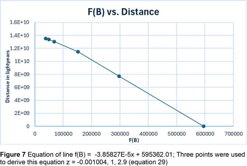
The equation for the relationship between f(B) and distance is:

f(B) = -3.85827E-5x + 595362.01 (equation 29) (Figure 7)

(Note): Because of the extreme velocities these equations are very sensitive to the number of significant digits that are used. This also leads to very abrupt changes like the abrupt change in the B value vs. redshift at .001, (Figure 12) (Figure 13) which will be discussed below. Therefore, the constants in Hammitt’s law will change slightly according to the number of significant digits that are used to derive the equation.

Notice that the equation for f(B) vs. distance is a linear equation with a negative slope, which is opposite of Hubble’s constant. This would be expected if blue shifted light was the inverse of redshifted light and redshifted light produced a positive slope. Figure 7 shows that the three of the points plotted on the graph form a linear line with the other three points all moving in the same direction away from the linear line created by the first three points. The three points that are not on the linear line are very distant objects. Therefore, it is assumed that these three points are not on the line because of assumptions in the 𝝠CDM theory.  

In the AMACS model Hammitt’s law which combines the equations from figure 6 and 7 to produce an equation that relates z value to distance is not a linear equation. It forms a hyperbolic curve with two asymptotes. One asymptote is at y = 15,430,802,147.08 light years. This would be the approximate distance to the CMB. This matches the initial assumption which was that the CMB was the very edge of the braneworld. Which is the observable universe we live in.

The other asymptote is well known in the fields of astronomy and cosmology z = -1. This is sometimes referred to as the blue wall because according to 𝝠CDM theory nothing can have a z value greater than -1. In the 𝝠CDM theory z = -1 refers to a point in the universe when the universe is no longer expanding but it is being compressed to form a point. It represents the absolute mathematical and physical limit for universal collapse. It is the exact threshold at which space itself would physically end in a "Big Crunch" scenario. AMACS theory also proposes that -1 is the limit to which light can be blue shifted for the same reason which is that the wavelengths of light cannot be compressed any further.

The hyperbolic curve that describes the asymptotes has two branches, a positive branch and a negative branch. The positive branch describes light up till the point that the front and trailing envelope arrive at the same time which is around z = -0.9966. Chart 3 shows how Δt is positive until -1 and then Δt switches signs and becomes negative. Therefore, the exact value in the AMACS theory would not be z = -1 like in the 𝝠CDM theory. It would be somewhere around z = -0.9966. The negative branch does not describe observations because any value in the negative branch would be moving backward in time.

Hammitt’s Law

The following three equations are three forms of Hammitt’s Law. Equations 30 and 31 are just different forms of the same equation. Equation 32 is a modified version of Hammitt’s Law adjusted to fit current 𝝠CDM theory distances.

x_AMASC = ((-15,369,582,740.45)/(z+0.9966)) + 15,430,802,147.08 (equation 30)

x_AMASC = ((15,430,802,147.08(z) + 8,752690.67))/(z+0.9966) (equation 31) (both equations give the same graph.

x_𝝠CDM = ((-14,112,357,184.78)/(z+0.994)) + 14514934379.82 (equation 32)

Equations 30 and 31 were derived from points whose distances could be measured by either cepheid variables, supernovae, or both.  Those points would be the first three points on figure 7 that form a linear line. In any six-day creation cosmology the expansion of the universe, if present, is negligible. These points were chosen to reduce the impact of the inflationary effects of 𝝠CDM theory. The two equations were then equated to create the Hammitt’s Law equation. Equation 32 is the modified version that aligns the CMB distance with 13.8 billion light-years, as suggested by 𝝠CDM theory. Equations 30 and 31 were solved in different ways but the CMB was calculated to be 15.416 billion light-years away in both equations.

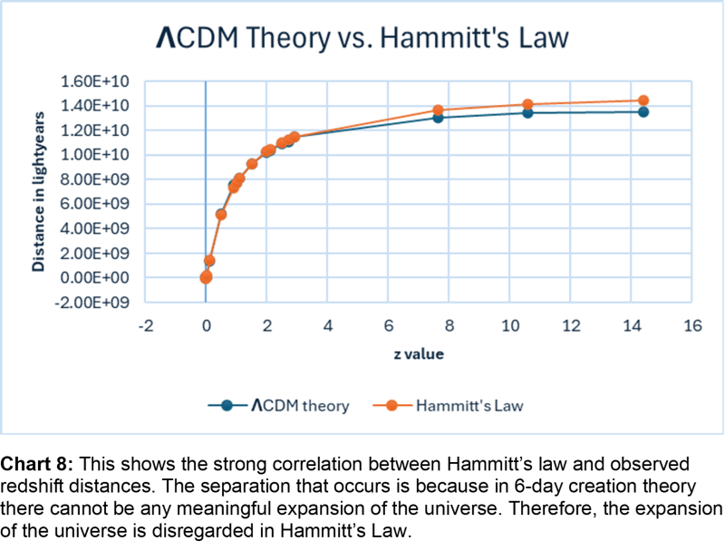
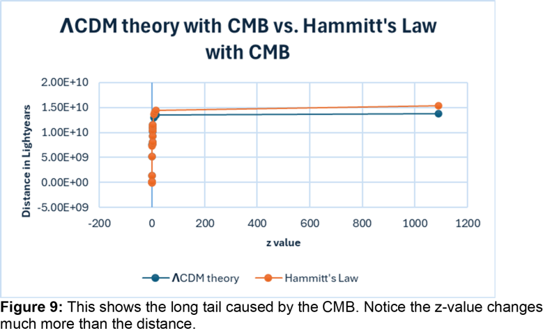
Figures 8 and 9

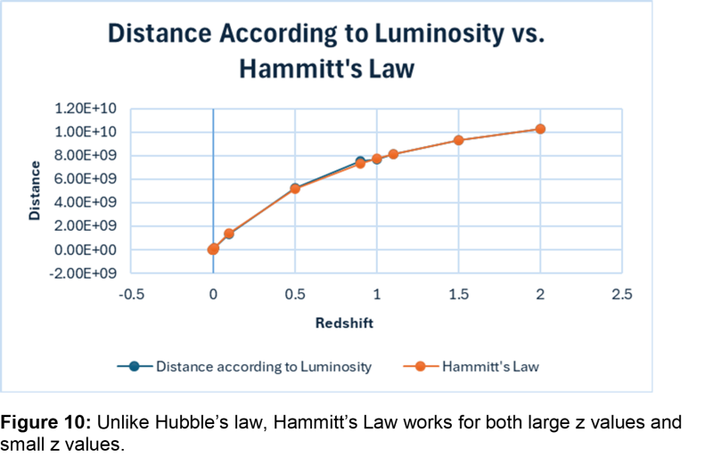
Figure 10 shows how Hammitt’s Law shows good correlation even at z values between 0 to 2 where distance has to be measured by luminosity.

Figure 10

The 13.8 billion years suggested by 𝝠CDM theory refers to a period marking the beginning of the universe, not a distance. According to 𝝠CDM theory, the universe's radius is approximately 45 billion light-years due to its ongoing expansion. In the early 1990s, prior to the discovery of "dark energy," cosmologists estimated the universe's age to be 15 billion years based on the ages of the oldest star clusters and stars, such as the Methuselah star.

The 𝝠CDM theory suggests that the current radius of the universe is approximately 45 billion light-years due to billions of years of expansion. Neither of these timelines aligns with a 6-day creation model. Previously, a radius of 15 billion light-years was considered a feasible size for the universe. Consequently, AMACS theory posits that God created the universe with a radius of about 15 billion light-years, which is the radius being calculated in this framework.

 

 

Hammitt’s Law Redshift to distance

Hammitt’s Law provides compelling support for the credibility of both AMASC theory and string theory overall. Hammitt’s law can make precise predictions regarding the redshift of stars and their distances based on the equations of string theory, without depending on 𝝠CDM theory. If the universe has a radius of 15 billion light years, then AMASC theory would be highly accurate in predicting the distances to any observable object simply by knowing the z value of that object. Even if Hammitt’s Law is not accepted it still could be used to estimate the distance to any observable object in the universe.

The AMASC model addresses not only the challenges related to the travel light problem in a six-day creation context but also resolves several issues in 𝝠CDM theory. If redshift is not tied to the universe's expansion, then dark energy is unnecessary to account for observations. Hammitt’s Law describes the redshift of light very accurately at close distances and at far distances. AMACS theory accurately describes distance as a function of the z value all the way to the CMB.

Figure 8-9 shows Hammitt's law strong correlation with current 𝝠CDM theory distances. Except where Hammitt’s law predicts that the original size of the universe is 15.4 billion light years instead of 𝝠CDM theory’s 13.8 billion light years. Figure 10 shows how Hammitt’s law also has good correlation with luminosity distance when z < 1.

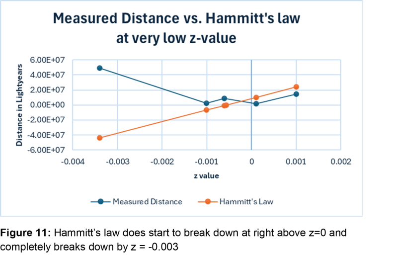
Figure 11 does show where Hammitt’s law does start to deviate from the observed values.

Figure 11

Hammitt’s law has a good correlation with luminosity distance all the way to z = 0.001835132 which is the critical value of B. It is at this point that Hammitt’s Law calculated distance becomes negative, yet the actual distance is positive. A similar abrupt change at a z value close to 0 is seen when the B value vs. z-value is graphed, which is shown in figure 17.

It seems that the jump in the B value would indicate that there is a combination of the motion of three different objects, the braneworld, the Earth and the object that is causing the blueshift. Hammitt’s law only accounts for the motion of one object on the braneworld, not two objects. It does seem plausible to create an equation that could account for the motion of more than one object on the braneworld but that would be for further research. Therefore, at the present time Hammitt’s law breaks down when redshift becomes negative.  

Reason for the redshift

Redshift in CMASC is caused for the same reason as in 𝝠CDM theory which is the expansion of the universe. However, 𝝠CDM theory has two different values for the expansion of the universe one rate for the older universe which is considered to have a redshift value >1. And a second value for the younger universe which is considered to have a redshift value < 1. (Trivedi 2022) (Bisnovatyi-Kogan and Nikishin, 2023) CMASC would be subject to this same tension along with all of the problems and mysteries associated with 𝝠CDM theory. Instantaneous travel of light in the CMASC theory would be strictly confined to the time of creation.

In AMASC theory, redshift is caused by the different velocities of the front and trailing envelopes.  Chart 1 shows the change in time between the front envelope and the trailing envelope with a radius of the compacted dimension of 1 x10^-35 m. This produces a T_dominante = 2.282 x 10^-40 seconds. T_dominante is the time it takes for the redshifted light to become dominant when compared to the blue shifted light. The next section will show how the z value changes with Δt. 

Arrival times forward and trailing envelops

The arrival time for the forward envelope to distance D is described by:

            t_forward(D) = D/v_eff (equation 33)

                        t_forward(D) = arrival time of the forward envelope

                        D = distance

                        v_eff = effective velocity

The arrival time for the trailing envelope at distance D:

            t_trailing(D) = D/w (equation 34)

                        t_trailing(D) = arrival time of trailing envelop

                        D = distance

                        w = velocity of trailing envelope

Equation 35 would be the time delay between the front and trailing envelopes. The forward time is subtracted from the trailing time so that time remains positive. The fact that the time is always positive is a key fact in this theory.  “An instantaneous round trip is possible but closed time-like curves are not. In short, there is no causality violation on the brane because the velocity of the return signal, while superluminal, is not superluminal enough (Greene et. Al. 2023).” Therefore, the broken Lorentz invariant in this theory is what makes Lisle's ACS theory plausible. However, the return trip does not have to be ½ the effective velocity it just has to be slower than the effective velocity in the AMACS model.   

            Δt(D) = t_trailing(D) - t_forward(D) = D(1/w - 1/v_eff)  (equation 35)

The trailing envelope that is redshifted keeps delivering redshifted images. The number of redshifted images increases per unit time and is roughly proportional to the size of the radius 1/R of the compacted dimension. This would be similar to wave length and frequency. If it is assumed that the cumulative energy from the trailing envelope grows linearly with Δt then the fraction of the total energy from the trailing envelope can be modeled by equation 36. 

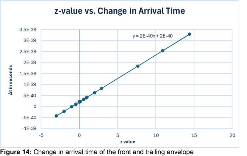
Figure 14

F(R) = Energy from trailing up to time t_trailing / Total energy from both envelopes (equation 36)  

If it is assumed that the energy flux from each envelope is constant the energy from the trailing envelope f(R) can be described by the following equation:

            f(R) = Δt(D) / (Δt(D) + t_char) (equation 37)

t_char = The characteristic time scale over which the forward envelope’s contribution is significant. This time scale would be related to the compacted dimension.

t_char = 2𝜋R/w (This would be the time needed to add one additional winding from the trailing envelope or in other words the time it takes for the light to “go around” the compacted dimension. The velocity of the trailing envelope is given by equation 38.

ω = -γ [(1 + Γ²B²β²) / (1 + Γ²Bγβ²)] (Greene et al., 2023) (equation 38)

Since the γ and β would be constants and B is also very close to being a constant value. ω remains relatively constant value across all calculations. It is interesting that ω does equal ½ of 𝛾 as long as the velocity of the moving object close to B critical.

Derivation of The Equation for Δt

The summation of the redshifted light and the blue shifted light caused by the difference in arrival time gives the effective z value. Equation 39 describes this summation. 

z_eff =(f(R)) (D_red) + (1- (fR)) (D_blue) (equation 39)

            D_red = 1088.92

            D_blue = -0.998165003

Solving equation 39 for f(R) gives equation 40. 

f(R) = (z - D_blue) / (D_red - D_blue) (equation 40)

Equation 40 shows that as z approaches 1088.92, f(R) approaches 1 and as z approaches -0.998165003_, f(R) goes to 0 and therefore Δt goes to 0.

If 2𝜋R/w is substituted for t_char in equation 37, then equation 37 becomes:

  f_red(R) = Δt(D) / (Δt(D) + 2𝜋R/w) (equation 41)

Solving equation 41 for Δt gives equation 42 which shows that when f(R) equals 1 the equation becomes undefined and as z approaches 1. Δt goes to infinity.  This occurs as z approaches 1089.92 or as light approaches the CMB which would represent the speed of the braneworld in the bulk.

 Δt = f(R)(2𝜋R/w) / (1- f(R)) (equation 42)

By utilizing equations 41 and 42, it can be seen in chart 3 how t_dominate correlates to a z value of -0.455. This is the point where the blue shifted light has faded enough so that the redshifted light can start to become dominant.

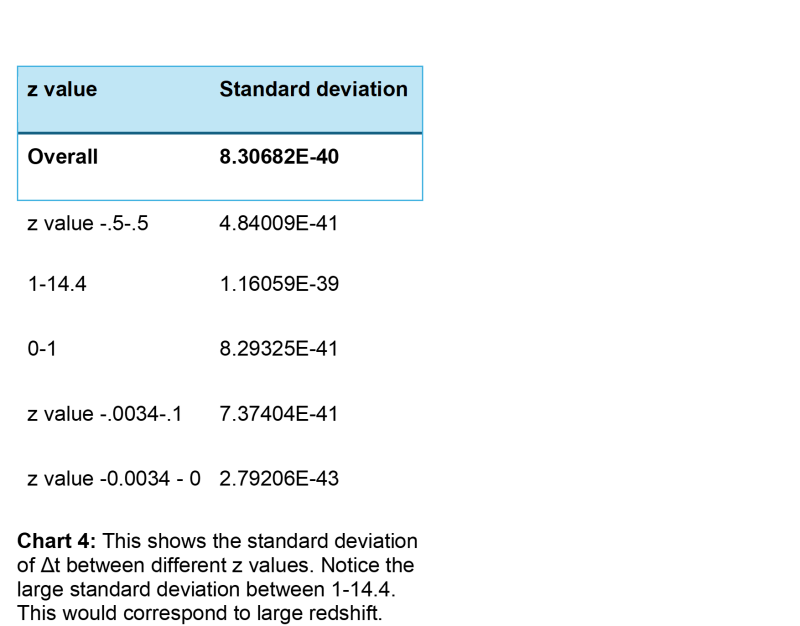
Hubble’s law describes the z values > 1 as nonlinear and z values ≪ 1 as linear. This is shown in the graphs that relate redshift to distance.  In 𝝠CDM theory z values > 1 would be because the expansion of the universe was greater when these stars and galaxies were formed. Charts 3 and 4 explain this observation according to AMACS theory. Chart 4 shows the standard deviation for Δt when objects have z-values of 1-14, is almost 2 orders of magnitude longer than the change in arrival time of objects with z values from 0-1. 

In 𝝠CDM theory, the z value represents the fractional change in wavelength and is defined by equation 41.

            z = (λ_obs - λ_emit) /λ_emit  (equation 43)

For z to have a value of -1 the 𝛾_obs would have to equal 0. Physically this signifies an object that is approaching at the speed of light. Therefore, -1 is theoretically possible, but no known astronomical object has a z value of -1 because it would require an object to be traveling at the speed of light relative to the observer. At this speed the wavelength is reduced to zero. Astronomers regularly observe objects with a negative z value. However, these z values are very close to zero not close to -1.

AMASC theory would describe the approach to z = -1 in a similar way. t_dominate occurs at z = -0.455 at this point the redshifted light would no longer be dominant and the light would be much brighter and shifted heavily towards the blue end of the spectrum, because the blue shifted light has more energy than the redshifted light. Light would appear very blue and very bright as z = -0.455 is approached because the reduction in Δt.  

Equation 43 describes 𝝠CDM theory’s view on redshift. 𝝠CDM theory describes redshift as when an object moves away from the Earth its wavelength of light will be stretched and it is this stretching that causes the light to be shifted towards the red. Most of the redshift effect is caused by the expansion of the universe. However, an object that has a particular velocity towards the Earth the light will be blue shifted and if an object has a particular velocity going away from the Earth it will be red shifted even more.  

AMASC theory proposes that the redshift of an object is a combination of the movement of the braneworld in the bulk and the particular motion of the object. The red shift that 𝝠CDM theory would tribute to expansion. AMASC theory would describe as a difference in arrival times between the front and trailing envelope. It is this difference in arrival times caused by the increased travel time which in turn is caused by an increase in distance.

At z = -0.998165003, Δt goes to infinity because of the combination of motion of the braneworld and the particular motion of the Earth. In other words, the trailing envelope has caught the front envelope. Therefore, AMASC theory would describe ≅ -1 as the point in which there is no time difference between the arrival time of the front and trailing envelope.

At a z value of -1 there are two things that occur. The B value becomes greater than the B critical value, B > B_critical and also Δt becomes positive indicating that the signal is going backward into time. 𝝠CDM theory describes this point as having a value of -1. AMASC theory value of z = -0.998165003 is only 0.18% from -1. Hammitt’s law predicts that this happens at -0.9966 which is .3% from -1. This is not just strong support for the AMASC theory and string theory but also for the connection of the CMB with blueshift limit of -1. String theory predicts an actual physical manifestation using the extra dimension and the movement of light strings as proposed in String Theory that matches observation! Chart 3 shows how Δt is negative up until the blueshift limit of -1.

For B > B_critical the signal propagation speed turns negative, which means the signal propagates backwards in time… Perhaps the superluminal signal velocity renders this outcome inevitable, but we still find it remarkable that simply having an extra compact spatial direction in an otherwise Lorentz invariant theory yields a controlled classical setting in which observers can send signals to the past. (Greene et al., 2023).

Dr. Greene describes how this could be used in the future. “One implication is the capacity for real time communication across arbitrarily large distances (Greene et al., 2023).” This idea will not be explored because it falls outside of this paper’s scope. However, it does show that Dr. Greene believes that instantaneous signals can be sent and even sent back into time and over very large distance instantaneously. However, one of the major issues with instantaneous signals is causality. 

Causality

Many physicists are troubled by the effective speed of light being greater than the actual speed of light because of the issues it causes with causality. Meaning that the effect would happen before the cause. That makes for good science fiction but not good science. Greene et al. address this apparent dilemma in his 2023 paper (Greene et al, 2023). Equation 6 describes the velocity of the front envelope. There can be no time difference when velocity goes to infinity because the trailing envelope also has to have an instantaneous velocity also.       

 

Equations 44 and 45 describe the velocity of the trailing envelope.

 (equation 44)

ω = -γ [(1 + Γ²B²β²) / (1 + Γ²Bγβ²)] (equation 45) (Greene et. al, 2023) 

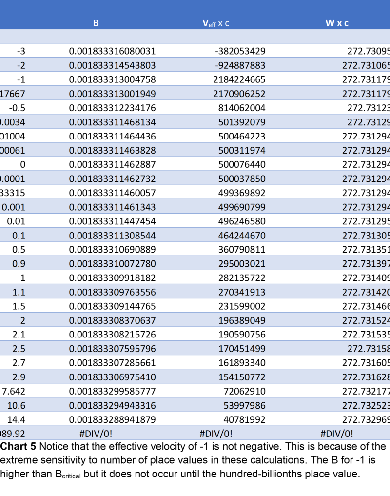
In this equation as B goes towards B_critical, ω goes towards -1/2γ. ω is always superluminal and moving in the opposite direction because γ is negative. γ is negative to indicate that this signal is traveling in the opposite direction as the effective velocity which is characteristic of a light cone. ω is always superluminal because of the boundaries that equation 45 places on ω.  When B = 0, which is an indication that the observer that is on the brane is not moving, v_eff is γ and ω is -γ. Which indicates that the velocity light in the backward direction is equal to the effective velocity in the forward direction. The light cone would propagate like a normal light cone. However, as the observer approaches the speed of light, B → 1, ω → 0 and v_eff → 0. However, v_eff would always be a little faster than ω because of the denominator in the v_eff equation. This is also shown on chart 5.

Chart 5

The following describes the total time elapsed for a trip that goes out and back to a point that is a distance D along the x axis.

t = D(1/v - 1/ω) = 2D/v_eff  (equation 46)(Greene et. al, 2023)

Solving this equation for the effective velocity results in the following.

            v_eff = 2(1/v - 1/ω)^-1 = γ (1 + Γ²B²β²) (equation 47)

In the equation above v_eff is always positive and is bounded below by v_eff ≥ γ and is unbounded above. Since v_eff is always positive it means that time also has to be always positive and is bounded below by 0 and bounded above by 2D/γ

            0 < T ≤ 2D/γ  (equation 48)

Therefore because “all roundtrip signals return to their starting location after a non-negative amount of elapsed time, obviating the possibility of causality-challenging closed time like curves(Greene et al. 2023).”

“An instantaneous round trip is possible but closed time-like curves are not. In short, there is no causality violation on the brane because the velocity of the return signal, while superluminal, is not superluminal enough (Greene et al. 2023).”

Conclusion

Many of the observations made by the James Webb space telescope are quickly making the Big Bang theory an untenable position to hold.

According to Fulvio Melia, “the discovery of well-formed galaxies at such an early stage in the history of the universe has been very disturbing for many astronomers and cosmologists, because nobody has a valid explanation for how they may have been formed. The work we are presenting makes the situation even more disconcerting for conventional cosmology, because it uses our most advanced scientific understanding to show that the stars in these galaxies are older than the universe itself, which makes no sense”.

𝝠CDM theory propose that it take a billion years for a galaxy to form. This puts a serious time limitation on the formation of the very early galaxies.

But the JWST observations have pushed the threshold for these processes too uncomfortably close to the Big Bang itself. We appear to have exhausted any flexibility left in understanding how the primordial plasma could have cooled and condensed rapidly enough to form these structures by ∼300 Myr in the context of ΛCDM (Melia 2023). Without much doubt, some significant new physics would be required to adequately explain how such massive structures could have formed so quickly in the ΛCDM Universe(Lisle 2024).

𝝠CDM theory does not just have problems with time but it also has problems with observations.

Thus, all other things being equal, galaxies should appear smallest at a distance corresponding to redshift 1.6 according to the standard model. Beyond that distance, galaxies should appear larger as their redshift increases. However, this effect is simply not seen in any Hubble Space Telescope (HST) or JWST images. Indeed, galaxies continue to appear smaller with increasing distance as if the large-scale spatial geometry of the universe were purely Euclidian as will be shown below. This is what we would expect if the Hubble law were due to Doppler shifts of galaxies moving through a non-expanding space(López-Corredoira 2024).

One of the unproven theoretical predictions of string theory is the extra and compacted dimensions. This study shows that by utilizing these compacted dimensions and the movement of strings an accurate cosmology that is consistent with observations can be formed. In this String Theory cosmology, the universe can have any age because the redshift of light is no longer a function of time and distance. It is simply a function of distance, the velocity of the braneworld in the bulk and the particular motion of the Earth on the braneworld. These movements break the Lorenzo invariant allowing for the front envelope of the light cone to travel at a different velocity than the trailing envelope. Therefore, causing a Δt in arrival times between the front and trailing envelopes, which increases the redshift of light.

The superluminal effective velocity of light is produced by the velocity of the braneworld in the bulk and the radius of the compacted dimension with the particular motion of the Earth. This motion produces a near instantaneous effective velocity of light from any point in the universe.

This model makes it possible for the universe to be any age and any size. Since in the AMACS model, redshift is not a function of time but of a difference in arrival times of light objects in the cosmos are being seen as they currently are not as they were billions of years ago. Therefore, String Theory would suggest that looking at stars and galaxies in the cosmos would not be looking back into time, but as they appear in real time.

 

 Bibliography

Answers in Genesis. “The Distant Starlight Problem: What Are the Possible Answers?” Accessed May 7, 2026. https://answersingenesis.org/astronomy/starlight/distant-starlight/.

Bisnovatyi-Kogan, G. S., and A. M. Nikishin. “Eliminating the Hubble Tension in the Presence of the Interconnection between Dark Energy and Matter in the Modern Universe.” arXiv:2305.17722. Preprint, arXiv, May 28, 2023. https://doi.org/10.48550/arXiv.2305.17722.

Dai, De-Chang, and Dejan Stojkovic. “Superluminal Propagation along the Brane in Space with Extra Dimensions.” The European Physical Journal C 84, no. 2 (February 2024): 175. https://doi.org/10.1140/epjc/s10052-024-12535-w.

Greene, Brian, Janna Levin, and Maulik Parikh. “Brane-World Motion in Compact Dimensions.” Classical and Quantum Gravity 28, no. 15 (August 2011): 155013. https://doi.org/10.1088/0264-9381/28/15/155013.

Greene, Brian, Daniel Kabat, Janna Levin, and Arjun S. Menon. “Superluminal Propagation on a Moving Braneworld.” Physical Review D 106, no. 8 (October 2022): 085001. https://doi.org/10.1103/PhysRevD.106.085001.

Greene, Brian, Daniel Kabat, Janna Levin, and Massimo Porrati. “Back to the Future: Causality on a Moving Braneworld.” Physical Review D 107, no. 2 (January 2023): 025016. https://doi.org/10.1103/PhysRevD.107.025016.

Humphreys, D. “New View of Gravity Explains Cosmic Microwave Background Radiation.” Journal of Creation 28, no. 3 (2014): 106–14. creation.com/articles/new-view-of-gravity.

Kabat, Daniel, and Marcelo Nomura. “Induced Lorentz Violation on a Moving Braneworld.” Physical Review D 108, no. 10 (November 2023): 105014. https://doi.org/10.1103/PhysRevD.108.105014.

Lisle, Jason. “Sizes of Galaxies in JWST Data Suggest New Cosmology.” Answers Research Journal 17 (July 2024): 445–57. https://answersingenesis.org/cosmology/jwst-data-suggest-new-cosmology/.

López-Corredoira, M., F. Melia, J. J. Wei, and C. Y. Gao. “Age of Massive Galaxies at Redshift 8.” The Astrophysical Journal 970, no. 1 (July 2024): 63. https://doi.org/10.3847/1538-4357/ad4f86.

Trivedi, Oem. “Another Look on the Connections of Hubble Tension with the Heisenberg Uncertainty Principle.” arXiv:2207.10570. Preprint, arXiv, December 2, 2022. https://doi.org/10.48550/arXiv.2207.10570.